This section is concerned with the solution of the generalized eigenvalue
problems  ,
,  , and
, and  , where
A and B are real symmetric or complex Hermitian and B is positive definite.
Each of these problems can be reduced to a standard symmetric
eigenvalue problem, using a Cholesky factorization of B as either
, where
A and B are real symmetric or complex Hermitian and B is positive definite.
Each of these problems can be reduced to a standard symmetric
eigenvalue problem, using a Cholesky factorization of B as either
 or
or  (
( or
or  in the Hermitian case).
In the case
in the Hermitian case).
In the case  , if A and B are banded then this may also
be exploited to get a faster algorithm.
, if A and B are banded then this may also
be exploited to get a faster algorithm.
With , we have

Hence the eigenvalues of are those of  ,
where C is the symmetric matrix
,
where C is the symmetric matrix 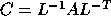 and
and  .
In the complex case C is Hermitian with
.
In the complex case C is Hermitian with  and
and  .
.
Table 2.13 summarizes how each of the three types of problem
may be reduced to standard form , and how the eigenvectors z
of the original problem may be recovered from the eigenvectors y of the
reduced problem. The table applies to real problems; for complex problems,
transposed matrices must be replaced by conjugate-transposes.
Table 2.13: Reduction of generalized symmetric definite eigenproblems to standard
problems
Given A and a Cholesky factorization of B,
the routines xyyGST overwrite A
with the matrix C of the corresponding standard problem
(see Table 2.14).
This may then be solved using the routines described in
subsection 2.3.4.
No special routines are needed
to recover the eigenvectors z of the generalized problem from
the eigenvectors y of the standard problem, because these
computations are simple applications of Level 2 or Level 3 BLAS.
If the problem is and the matrices A and B are banded,
the matrix C as defined above is, in general, full.
We can reduce the problem to a banded standard problem by modifying the
definition of C thus:

where Q is an orthogonal matrix chosen to ensure that C has bandwidth no greater than that of A. Q is determined as a product of Givens rotations. This is known as Crawford's algorithm (see Crawford [14]). If X is required, it must be formed explicitly by the reduction routine.
A further refinement is possible when A and B are banded, which halves
the amount of work required to form C (see Wilkinson [79]).
Instead of the standard Cholesky factorization of B as  or
or  ,
we use a ``split Cholesky'' factorization
,
we use a ``split Cholesky'' factorization  (
( if B is complex), where:
with  upper triangular and
  lower triangular of
order approximately n / 2;
S has the same bandwidth as B. After B has been factorized in this way
by the routine
xPBSTF ,
the reduction of the banded generalized
problem to a banded standard problem
is performed by the routine xSBGST
(or xHBGST for complex matrices).
This routine implements a vectorizable form of the algorithm, suggested by
Kaufman [57].
lower triangular of
order approximately n / 2;
S has the same bandwidth as B. After B has been factorized in this way
by the routine
xPBSTF ,
the reduction of the banded generalized
problem to a banded standard problem
is performed by the routine xSBGST
(or xHBGST for complex matrices).
This routine implements a vectorizable form of the algorithm, suggested by
Kaufman [57].
--------------------------------------------------------------------
Type of matrix                    Single precision  Double precision
and storage scheme   Operation    real     complex  real     complex
--------------------------------------------------------------------
symmetric/Hermitian  reduction    SSYGST   CHEGST   DSYGST   ZHEGST
--------------------------------------------------------------------
symmetric/Hermitian  reduction    SSPGST   CHPGST   DSPGST   ZHPGST
(packed storage)
--------------------------------------------------------------------
symmetric/Hermitian  split        SPBSTF   CPBSTF   DPBSTF   ZPBSTF
banded               Cholesky
                     factorization
--------------------------------------------------------------------
                     reduction    SSBGST   DSBGST   CHBGST   ZHBGST
--------------------------------------------------------------------